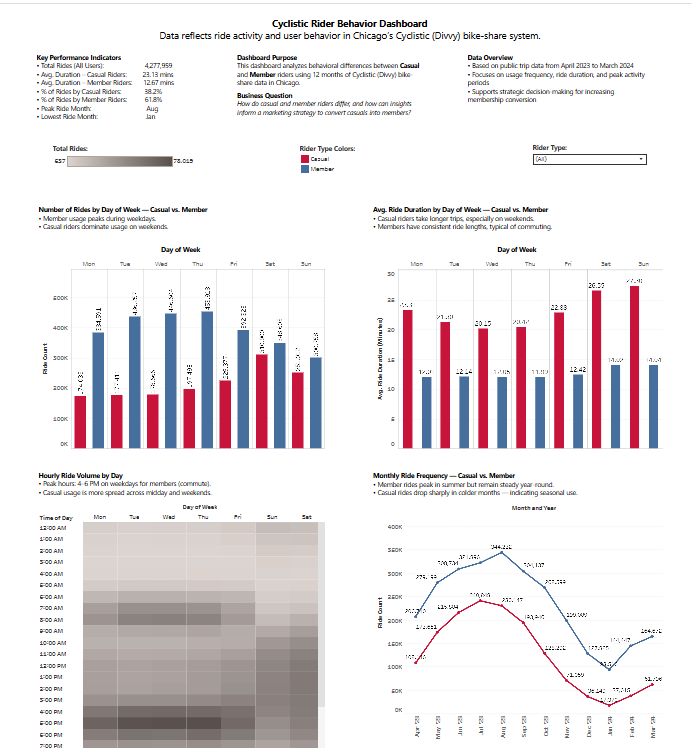
← Back to Portfolio
Data Analytics Capstone R Programming Tableau tidyverse Behavior Analytics

Cyclistic Rider Behavior Analysis

A year-long analysis of Chicago's Cyclistic bike-share program comparing casual riders and annual members. This capstone project follows the full Google Data Analytics process to inform marketing strategies that convert high-usage casual riders into long-term members.

12
Months
Full year of trip data
4.2M
Cleaned rides
Row volume after preprocessing
2
Rider types
Casual and annual members
5
Day window
Upper bound for ride length checks
5
Core views
Rider mix, trends, duration analysis
Rider Segmentation & Behavior Patterns Usage Trends & Seasonality Analysis Membership Growth Strategy

Project overview

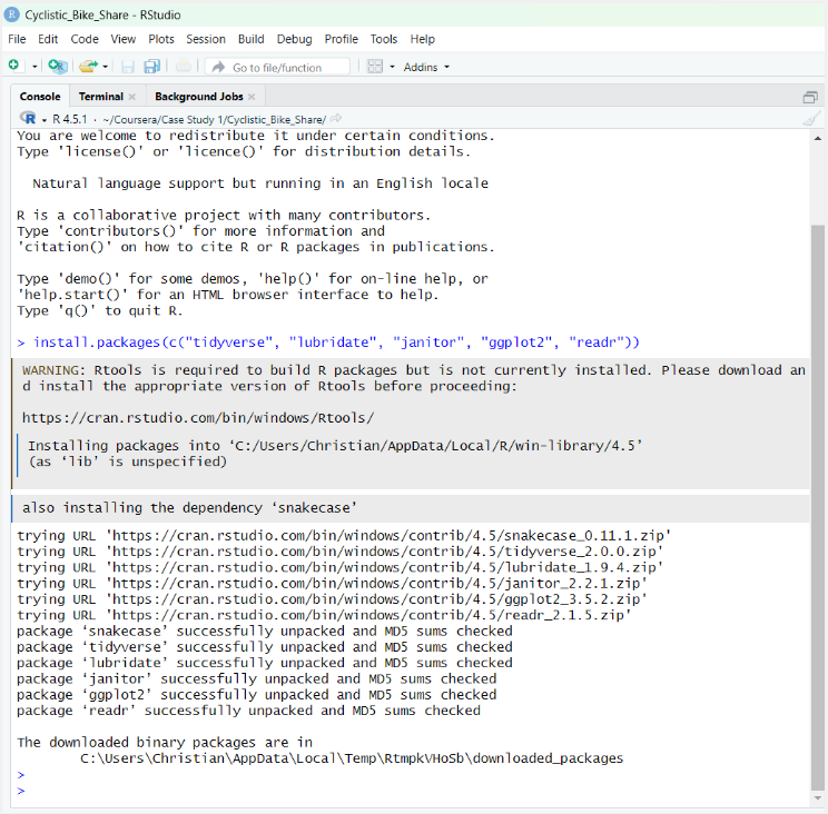
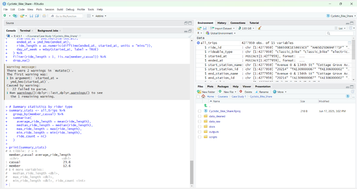
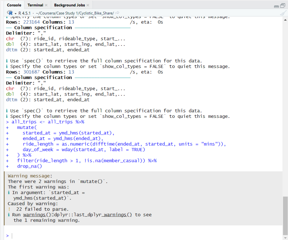
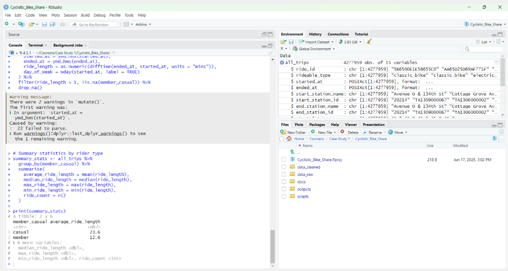
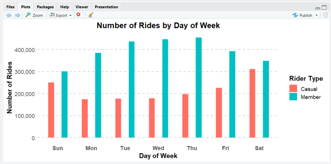
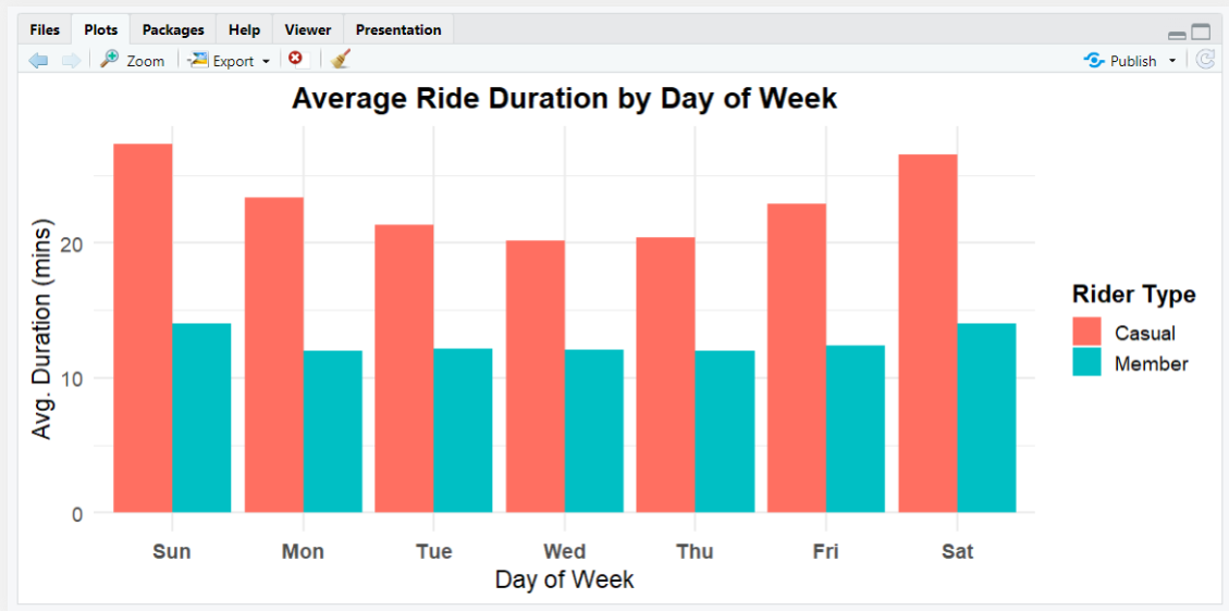
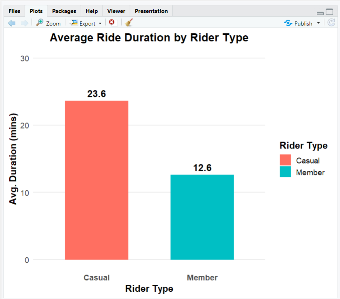
Combined 12 months of Cyclistic trip data from Chicago to uncover behavioral differences between casual riders and annual members. Using R (tidyverse, lubridate, janitor, ggplot2) for preparation and analysis, plus Tableau for visualization, explored ride volume, duration and timing patterns across seasons and weekdays.

Key deliverables

  • Merged and cleaned 12 months of Divvy/Cyclistic trip data using tidyverse
  • Engineered ride_length and day_of_week features for segmentation
  • Computed summary statistics comparing ride behavior between rider types
  • Developed ggplot2 visuals and Tableau dashboard to surface trends
  • Produced concrete recommendations to increase membership conversion

Workflow Overview

Phase 1

Import & Standardization

Downloaded and combined 12 monthly CSVs using read_csv(), map_df() and clean_names().

Phase 2

Cleaning

Removed invalid rides, parsed timestamps and dropped rows with missing data.

Phase 3

Feature engineering

Engineered ride length, weekday labels and features for behavioral segmentation.

Phase 4

Analysis

Summarized rides by rider type, weekday and season to reveal core patterns.

Phase 5

Visualization

Created ggplot2 charts and Tableau dashboard for stakeholder storytelling.

Lab Breakdown

Phase 1 — Importing and standardizing 12 months of Cyclistic data

The project begins by downloading 12 monthly CSVs from the Divvy/Cyclistic portal. Using tidyverse, these files were imported and combined into a single, clean dataframe ready for analysis.

1.1 — Package setup and environment readiness

RStudio was configured with tidyverse, lubridate, janitor, ggplot2 and readr to support the full workflow from import through visualization.

  • Installed and loaded tidyverse, lubridate, janitor, ggplot2 and readr
  • Verified versions and library paths for reproducibility
  • Created dedicated project folder with data directories
RStudio package installation

RStudio console confirming successful installation of required packages.

1.2 — Combining 12 CSVs into one dataframe

Using list.files(), map_df() and clean_names(), the 12 monthly CSVs were imported and standardized into one dataframe with normalized column names.

  • Collected file paths from the data_raw directory
  • Used map_df(read_csv) to stack monthly datasets
  • Cleaned column names with clean_names() for consistency
Data import and merge

RStudio environment after successfully importing and combining 12 months of trip data.

Phase 2 — Data cleaning and feature engineering

After import, focus shifted to removing invalid records and creating features that explain rider behavior. Using lubridate and dplyr, ride length and weekday labels were built.

2.1 — Cleaning timestamps and durations

Start and end timestamps were parsed into datetime objects, then used to calculate ride duration in minutes. Invalid rides were removed to avoid skewed averages.

  • Converted started_at and ended_at with ymd_hms()
  • Computed ride_length as numeric difference in minutes
  • Filtered out rides with duration ≤ 1 minute
Data cleaning transformation

RStudio console showing mutation steps for ride length and weekday plus filters for invalid rides.

2.2 — Engineering behavioral features

To support segmentation, day_of_week labels were created and used to compare weekday commuting patterns with weekend leisure trips across rider types.

  • Derived day_of_week from started_at using wday()
  • Classified rides into weekday versus weekend groupings
  • Retained only records with valid member_casual labels
Feature engineering

Feature engineering snippet adding ride length and weekday labels to the combined dataset.

Phase 3 — Summary statistics and trend analysis

With a clean dataset, behavior was summarized by rider type, weekday and season. These statistics reveal that casual riders take longer trips concentrated on weekends while members ride more on weekdays.

3.1 — Comparing ride duration and volume by rider type

Using group_by() and summarise(), mean, median, min and max ride length were computed for each rider segment along with total ride counts.

  • Casual riders show longer average ride durations than members
  • Members complete more rides overall despite shorter trips
  • Summary metrics serve as inputs to dashboard KPIs
Summary statistics

Summary statistics showing ride length and volume for casual and member riders.

3.2 — Weekday and seasonal patterns

Additional aggregations by weekday and month surfaced clear seasonality: casual riders cluster in warmer months and on weekends, while member activity resembles workweek commute patterns.

  • Built weekday summaries for ride counts and average duration
  • Mapped peaks in casual usage to summer weekends
  • Confirmed steady weekday usage by members consistent with commuting
Rides by day of week

Rides by day of week: casual volume spikes on weekends, member volume peaks Monday-Friday.

Phase 4 — Visualization and communication

Visualization combines R-based exploration with a polished Tableau dashboard. ggplot2 charts help iterate on questions while Tableau delivers an interactive view for stakeholders.

4.1 — Core ggplot2 visuals

In R, bar charts were created comparing ride counts and average duration by weekday and rider type. These plots validate behavioral patterns before investing in dashboard design.

  • Rides by day of week split by rider type
  • Average ride duration by weekday and segment
  • Overall average ride duration by rider type
Average duration by weekday

Average ride duration by day of week showing longer casual rides on weekends.

Average duration by rider type

Average ride duration by rider type: casual riders stay out nearly twice as long as members.

Sample R scripts — from raw CSVs to enriched dataset

These snippets show how the analysis flows from package setup through import, cleaning, summary statistics and plotting. They mirror the structure of the Cyclistic case study.

Package setup and import

install.packages(c("tidyverse","lubridate","janitor"))

library(tidyverse)
library(lubridate)
library(janitor)

file_list <- list.files("data_raw", pattern = "*.csv")

all_trips <- file_list %>%
  map_df(read_csv) %>%
  clean_names()

Cleaning and feature engineering

all_trips <- all_trips %>%
  mutate(
    ride_length = difftime(ended_at, started_at),
    day_of_week = wday(started_at, label = TRUE)
  ) %>%
  filter(ride_length > 1) %>%
  drop_na()

summary_stats <- all_trips %>%
  group_by(member_casual) %>%
  summarise(avg = mean(ride_length))

Phase 5 — Dataset pipeline and Tableau dashboard

The final phase packages the cleaned dataset for Tableau, where stakeholders can explore rider behavior, filter by segment and drill into KPIs that tie directly to membership growth strategy.

Dataset and processing pipeline

  • 12 monthly CSVs — raw trip logs from Divvy/Cyclistic portal
  • R tidyverse pipeline — imports, cleans and standardizes records
  • Feature engineering — ride length, weekday labels and metrics
  • Aggregated summaries — casual vs member behavior across time
  • Tableau export — cleansed dataset feeds the dashboard

Data flow into Tableau

  • RStudio → save cleaned .csv file with engineered features
  • Tableau Desktop → connect to cleaned dataset as data source
  • Build worksheets for ride volume, duration and rider mix
  • Combine worksheets into dashboard with filters for rider type and weekday
  • Publish to Tableau Public for interactive exploration

Cyclistic Rider Behavior Dashboard (Tableau)

The Tableau dashboard summarizes 12 months of rider behavior, comparing casual and member riders with filters for rider type, day of week and hour of day.

Tableau dashboard

Tableau dashboard combining ride volume, duration and seasonal trends to support membership decisions.

Rider Behavior Overview

The final dashboard delivers a consolidated view of Cyclistic usage, highlighting how casual riders and members differ by volume and duration. The metrics below summarize the year-long dataset.

4.17M

Total rides: combined casual and member trips after cleaning.

2.32M

Member rides: volume associated with annual subscribers.

1.85M

Casual rides: pay-per-ride and day pass usage.

26.7

Avg duration casual: minutes per trip for casual riders.

12.5

Avg duration member: minutes per trip for members.

Cyclistic dashboard

Visual summary of Cyclistic rider behavior split by rider type, weekday and season.

Rides by weekday

Weekday distribution showing casual weekend peaks and member weekday consistency.

Key Behavior Patterns

6 KEY INSIGHTS
WEEKEND LEISURE RIDERS

Casual usage spikes on weekends and in warmer months, suggesting leisure or tourism service use.

WEEKDAY COMMUTE PATTERNS

Members ride consistently on weekdays with shorter, repeatable trips aligning with commuting.

DURATION GAP

Casual riders spend nearly twice as long per ride as members, indicating different use cases.

CONVERSION OPPORTUNITY

High-frequency casual riders could be targeted with tailored membership offers.

SEASONALITY AWARE PRICING

Promotions timed to peak casual months can nudge repeat users toward memberships.

DASHBOARD STORYTELLING

The dashboard turns millions of records into a simple story supporting marketing decisions.

Growth and Retention Strategy

Tier 1: Acquisition

Objective: Convert high-usage casual riders into entry-level members.

  • Weekend membership promos Offer time-limited discounts for riders who take multiple weekend trips.
  • In-app conversion nudges Trigger messages like "You have taken 3 rides this week — save with membership".
  • Tourist bundles Create day or weekend bundles introducing casual riders to membership benefits.

Tier 2: Retention

Objective: Keep members engaged through consistent value and convenience.

  • Commute-friendly features Highlight dock availability, route suggestions and time savings for weekday trips.
  • Usage-based rewards Offer perks for members who hit monthly ride milestones.
  • Churn early warning Monitor drops in member usage and trigger retention campaigns.

Tier 3: Operations

Objective: Use behavioral data to keep the system efficient and rider-friendly.

  • Bike redistribution planning Align rebalancing with known weekday and weekend hot spots.
  • Demand forecasting Use historical patterns to anticipate high traffic days and congestion.
  • Continuous KPI monitoring Track ride volume, duration and member mix as ongoing health indicators.

Key insights

  • Casual riders show strong weekend and warm season peaks, reflecting leisure usage.
  • Members ride consistently on weekdays with shorter, utility-focused trips.
  • Average ride duration for casual riders is nearly double that of members.
  • Segmentation by rider type, weekday and season creates clear campaign levers.
  • Combining R and Tableau provides a repeatable pattern for data-driven decisions.

Skills demonstrated

R Programming Data Wrangling Feature Engineering ggplot2 Visualization Tableau Dashboards Behavior Analytics Cohort Segmentation Data Cleaning

Summary

This Cyclistic rider analysis connects raw open trip data to concrete membership strategy. By importing and cleaning 12 months of rides in R, engineering features for segmentation, and surfacing patterns in Tableau, the project delivers a clear picture of when and how different riders use the system — creating a natural path for targeted conversions, retention campaigns and operations planning grounded in real behavior.