Machine Learning Lab Python Scikit Learn Pandas SHAP Customer Analytics

Telco Customer Churn Analysis

Used a public telecom dataset to model which subscribers are likely to cancel service, then explained the drivers behind that risk so a retention team can step in before customers leave.

79.8%

Accuracy

Correct predictions

91%

Recall (Stay)

Non-churners correctly identified

49%

Recall (Churn)

Churners detected

66%

Precision (Churn)

Accuracy of churn predictions

26.5%

Churn Rate

Portion of churners

End to end churn modeling in Jupyter Random Forest with SHAP explainability Business ready retention insights

Project overview

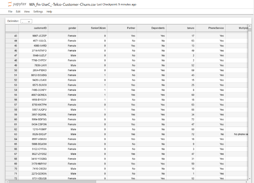
The lab uses a real telecom customer file where each row represents one account with service history, product bundle, billing behavior and a churn label. This raw table was transformed into a supervised learning pipeline that predicts churn and explains why some customers are at higher risk.

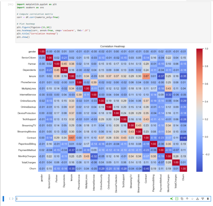
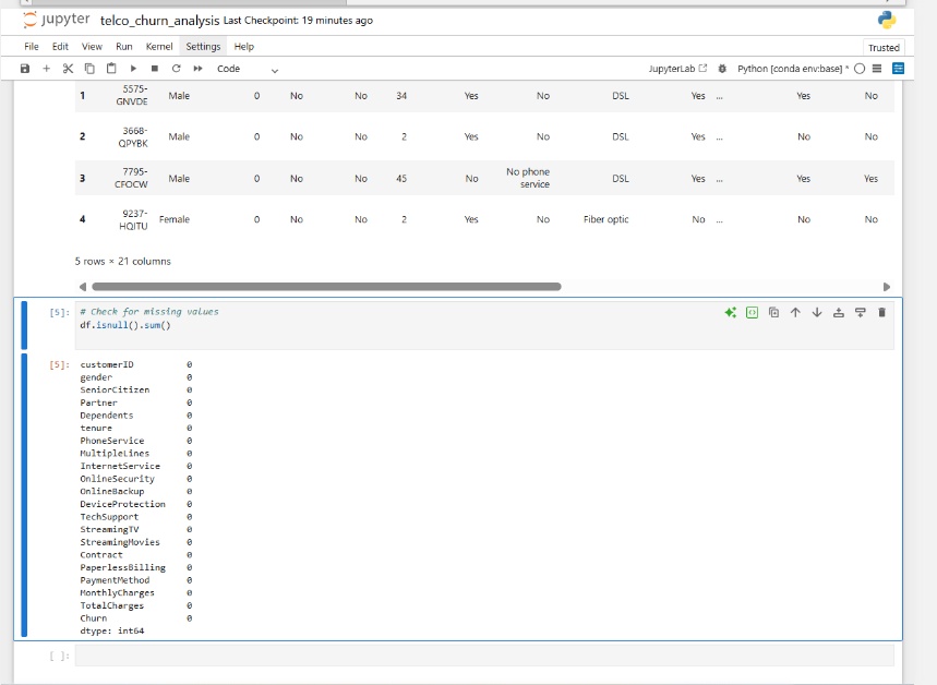
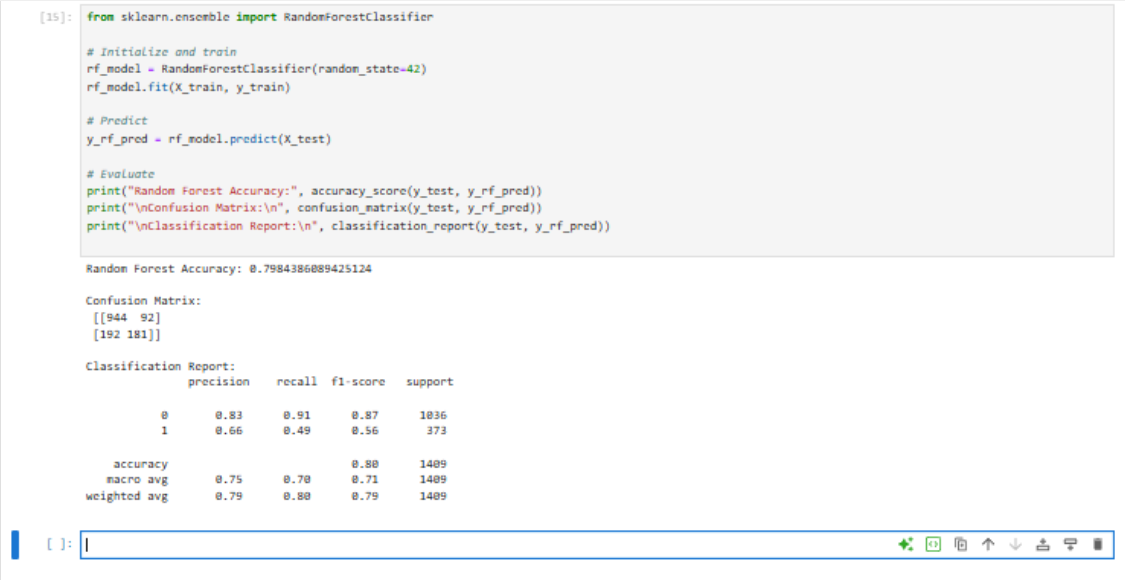
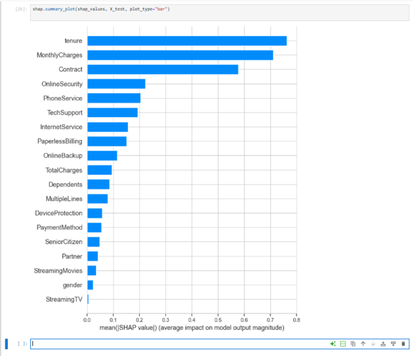
After cleaning billing fields and encoding plan details into numeric features, a Random Forest classifier was trained and its performance was compared to a logistic baseline. SHAP values then translated model output into a ranked list of churn drivers that can feed marketing and service playbooks.

Key deliverables

Notebook based workflow from raw CSV to trained model
Data cleaning steps that fix billing fields and remove incomplete records
One hot encoded feature set that preserves plan and service information
Random Forest classifier tuned and evaluated on a separate test split
Confusion matrix and classification report for both churn and non churn classes
SHAP summary plots that rank the strongest churn drivers for the business

Workflow Overview

Step 1

Data intake

Loaded the customer file into pandas, checked schema, row count and basic distributions.

Step 2

Cleaning

Fixed the TotalCharges field, handled missing entries and removed unreliable records.

Step 3

Feature prep

Encoded categorical columns, separated the churn label and built the final feature matrix.

Step 4

Modeling

Trained a Random Forest classifier and compared results with a logistic baseline.

Step 5

Explainability

Used SHAP to see which features push churn risk higher or lower for each customer.

Lab Breakdown

Phase 1 — Exploring the raw customer file

The notebook begins with a simple question: what does each row represent and which fields might help predict churn. It was confirmed that every record maps to a single customer and that the file includes service portfolio, contract style, billing amounts and a churn outcome.

1.1 — Inspecting the table in Jupyter

A quick head view in Jupyter shows the structure of the dataset: customer identifier, demographic attributes, service flags for internet and phone products, contract terms and the churn flag. This check confirms that the import ran correctly and that the data lines up with the documentation from the provider.

Verified column order, dtypes and row count
Confirmed that each customer has one record
Identified target column Churn for modeling

Preview of the raw telco churn dataset inside Jupyter before any cleaning.

1.2 — Correlation heatmap of numeric fields

To get an early feel for signal strength, a correlation matrix was created across numeric features and the churn flag. Tenure shows a clear negative relationship with churn, while higher monthly charges and certain contract patterns lean toward higher risk.

Converted the frame to numeric only for the heatmap
Used seaborn to plot correlations and spot strong links
Flagged tenure and billing features as promising signals

Correlation heatmap of numeric variables, including the churn label.

Phase 2 — Cleaning and fixing billing fields

Before any modeling, the file needed a small amount of repair. The main issue sits in the TotalCharges column, which arrives as text and includes blank entries for new customers.

2.1 — Converting TotalCharges and dropping incomplete records

TotalCharges was cast to a numeric type and invalid strings were turned into missing values. Those rows were then removed so the model only trains on customers with a consistent billing history. The customer identifier column was also dropped since it carries no predictive value.

df["TotalCharges"] = pd.to_numeric(df["TotalCharges"], errors="coerce")
df = df.dropna()
df = df.drop(columns=["customerID"])

A quick null count after this step confirms that all remaining fields are complete and ready for feature engineering.

Notebook cell that converts TotalCharges, drops missing rows and removes identifiers.

Phase 3 — Feature engineering and train test split

Most columns in the telco file are categories such as Yes or No, internet plan types or contract names. These need to become numeric while keeping their original meaning intact.

3.1 — One hot encoding churn features

Pandas get_dummies was used to apply one hot encoding to every categorical column, dropping the first level to avoid redundant dummy variables. The churn flag becomes Churn_Yes, which serves as the target label for modeling.

df_encoded = pd.get_dummies(df, drop_first=True)

X = df_encoded.drop("Churn_Yes", axis=1)
y = df_encoded["Churn_Yes"]

3.2 — Building a balanced train test split

To keep the churn rate consistent between training and evaluation, train_test_split was used with stratification on the target. This prevents the model from seeing a very different churn mix at training time than it will see at scoring time.

X_train, X_test, y_train, y_test = train_test_split(
    X, y,
    test_size=0.2,
    random_state=42,
    stratify=y
)

Phase 4 — Random Forest modeling and evaluation

With features in place, modeling moved forward using a Random Forest classifier. This ensemble balances flexibility and interpretability and usually performs well on structured customer data.

4.1 — Training the Random Forest classifier

The model trains on the full feature set with a modest depth and tree count so that the pattern remains general rather than memorizing the training customers.

rf_model = RandomForestClassifier(
    n_estimators=300,
    max_depth=12,
    random_state=42
)

rf_model.fit(X_train, y_train)
y_rf_pred = rf_model.predict(X_test)

Accuracy on the test set lands just under eighty percent, with stronger recall for customers who stay and moderate recall for customers who churn.

Random Forest accuracy, confusion matrix and classification report from the notebook.

Evaluation code

print("Random Forest Accuracy:", accuracy_score(y_test, y_rf_pred))
print("\nConfusion Matrix:\n", confusion_matrix(y_test, y_rf_pred))
print("\nClassification Report:\n", classification_report(y_test, y_rf_pred))

The confusion matrix shows 944 true retainers and 181 true churners correctly identified. Precision for the churn class is around sixty six percent, with recall near forty nine percent, which means the model favors catching many churners while keeping false alarms at a manageable level.

Phase 5 — SHAP driven explainability and business insight

Accuracy is useful, but a business team also needs to know why the model flags a customer as high risk. SHAP values provide that missing piece by attributing each prediction to individual features.

5.1 — Computing SHAP values for the Random Forest

The tree based SHAP explainer was used, which handles ensemble models efficiently. For every customer in the test set it returns a contribution score per feature, showing how that feature moves churn probability up or down.

explainer   = shap.TreeExplainer(rf_model)
shap_values = explainer.shap_values(X_test)

shap.summary_plot(shap_values[1], X_test)
shap.summary_plot(shap_values[1], X_test, plot_type="bar")

The bar style summary ranks global feature importance, while the main plot shows how low or high values of each feature influence churn risk.

SHAP summary plot where tenure, monthly charges and contract style emerge as leading churn drivers.

Interpreting the top churn drivers

Tenure

Shorter tenure pushes churn risk higher which reflects new customers who have not built loyalty yet. Long term customers rarely appear in the high risk group.

Monthly charges

Expensive plans raise churn risk, especially when combined with simple contract terms. Targeted discounts toward these customers can protect revenue.

Contract and support features

Month to month contracts and lack of support services trend toward higher risk, while long term contracts with security and technical support keep customers more stable.

Model Performance Overview

The trained Random Forest reaches roughly eighty percent accuracy on the test set and balances performance between churn and non churn classes. The model recognizes most customers who stay, while still catching nearly half of customers who leave which is enough to support focused outreach.

Confusion matrix and classification report summarizing how well the model distinguishes churn and non churn customers.

79.8%

Accuracy

Share of correct predictions

91%

Recall (Stay)

Non churn customers identified

49%

Recall (Churn)

Churners caught by model

66%

Precision (Churn)

Accuracy of churn predictions

26.5%

Churn Rate

Observed churn share

Retention Strategy Highlights

6 KEY IDEAS

EARLY TENURE OUTREACH

Focus retention campaigns on customers with short tenure who carry higher modeled risk.

PRICING SENSITIVITY

High monthly charges are a strong driver of churn so discounts or plan reviews for that segment can reduce loss.

CONTRACT DESIGN

Moving customers from month to month to longer contracts with valuable add ons can make the relationship more stable.

SUPPORT BUNDLES

Security and technical support services appear protective so they are good candidates for targeted cross sell.

PLAYBOOK TEMPLATES

High risk customers can follow a standard outreach play that blends proactive service checks and tailored offers.

CYCLE OF IMPROVEMENT

New outcomes can feed back into the model, sharpening feature importance and improving the targeting strategy over time.

Key insights

Tenure, monthly charges and contract style are the strongest global indicators of churn risk.
Even a simple tree ensemble can deliver almost eighty percent accuracy with clear business signal.
Targeting short tenure, high price customers yields the greatest opportunity for retention wins.
SHAP based explanations make a complex model understandable for non technical stakeholders.
Clean feature engineering and stratified splits are crucial for honest evaluation in churn work.

Skills demonstrated

Python Data Analysis Pandas Data Cleaning Feature Engineering Scikit Learn Classification Confusion Matrix Evaluation SHAP Model Explainability Customer Churn Analytics Storytelling With Notebooks

Summary

This telco churn lab walks from raw customer records to a production style modeling pipeline that flags at risk subscribers and explains why they might leave. Along the way it shows how careful cleaning, solid feature engineering, stratified splits and honest evaluation combine into a reliable classifier. SHAP based insights bridge the gap between data science and decision making so marketing and service teams can act with confidence on the model's signals.

← Back to Portfolio